Usage examples#

[2]:

from urllib.request import urlretrieve
import tempfile

import numpy as np
import matplotlib.pyplot as plt
import pennylane as qml
from scipy.stats import unitary_group

[3]:

from qutree import BBT

Bell state preparation#

[4]:

@qml.qnode(qml.device("default.qubit", wires=2))
def bell(t):
    qml.Hadamard(wires=[0])
    qml.CRY(np.pi*t,wires=[0,1])
    return qml.state()

ts = np.linspace(0,1,21)
Ss = np.array([bell(t) for t in ts]).T

[5]:

bbt = BBT(2)
bbt.add_data(Ss)
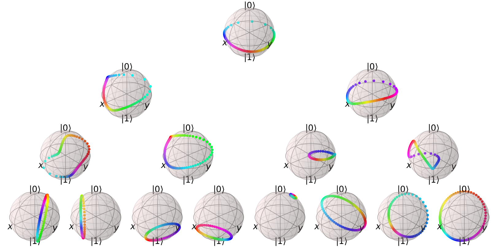
bbt.plot_tree()

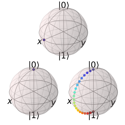
The top sphere shows the effect of the hadamard gate : an even superposition between the two basis state without phase offset. Then on the bottom sphere we wee the effect of the parametrised Control Y rotattion : The left sphere represent the subspace where the first qubit is 0. it is of course untouched by the CY gate. The right sphere represent the subspace where the first qubit is 1. The state is gradually rotated about the Y axis from 0 (blue) to 1 (red). The bell state corresponds to the red point.

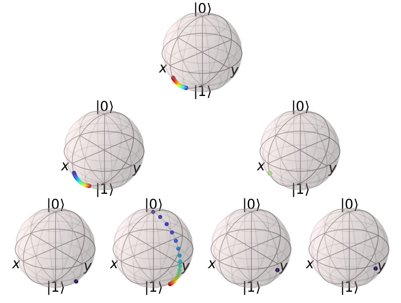
Study how an encoding spans the hilbert space#

[6]:

dev = qml.device('default.qubit', wires=3)

@qml.qnode(dev)
def circuit(t):
    state = np.array([1, 2j, 3, t*1j, 5, 6j, 7, 8j])
    state = state / np.linalg.norm(state)
    qml.MottonenStatePreparation(state_vector=state, wires=range(3))
    return qml.state()

print(qml.draw(circuit, expansion_strategy="device", max_length=80)(4))

0: ──RY(2.35)─╭●───────────╭●──────────────╭●────────────────────────╭●
1: ──RY(2.09)─╰X──RY(0.21)─╰X─╭●───────────│────────────╭●───────────│─
2: ──RY(1.88)─────────────────╰X──RY(0.10)─╰X──RY(0.08)─╰X──RY(0.15)─╰X

──╭●────────╭●────╭●────╭●─┤  State
──╰X────────╰X─╭●─│──╭●─│──┤  State
───RZ(1.57)────╰X─╰X─╰X─╰X─┤  State

[7]:

ts = np.linspace(0,8,21)
Ss = np.array([circuit(t) for t in ts]).T

[8]:

bbt = BBT(3)
bbt.add_data(Ss)
bbt.plot_tree()

quantum states dataset from Machine Learning#

The data is generated using the demo from pennylane about classification that can be found here : https://pennylane.ai/qml/demos/tutorial_variational_classifier.html

[9]:

# read the file from data folder in github
with tempfile.NamedTemporaryFile() as tmp:
    url = 'https://raw.githubusercontent.com/alice4space/qutree/main/docs/source/examples/data/iris_quantum_kernel.npy'
    urlretrieve(url, tmp.name)
    states_ml = np.load(tmp.name,allow_pickle=True)

[10]:

bbt = BBT(4)
lam = 0.3
cs = np.concatenate([np.random.random(50)*lam,np.random.random(50)*lam+1-lam])
bbt.add_data(states_ml.T,colors=cs)
bbt.plot_tree()

hamiltonian simulation#

[11]:

num_qubits = 4
U = unitary_group.rvs(2**num_qubits,random_state = 0)
D,S = np.linalg.eigh(U)

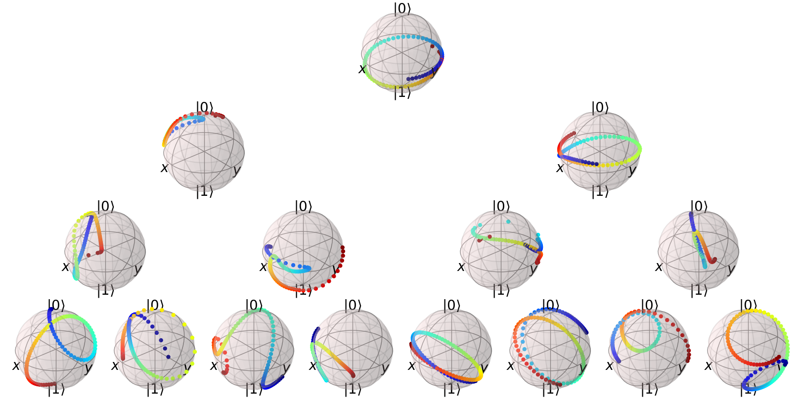
excite only two eigenstates : a single frequency#

[12]:

ka = 12
kb = 2

S0 = (S[:,ka]+S[:,kb])/np.sqrt(2)
Sts = []
ts = np.linspace(0,2*np.pi/np.abs(D[ka]-D[kb]),101)
for t in ts:
    Sts.append(S @ np.diag(np.exp(1j*D*t)) @ S.T.conj() @ S0)
Sts = np.array(Sts).T

[13]:

bbt = BBT(4)
bbt.add_data(Sts,cmap='hsv')
bbt.plot_tree()

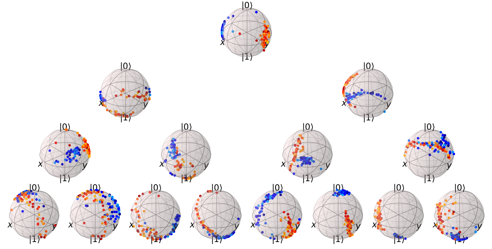
excite three eigenstates : three frequencies#

[14]:

ka = 12
kb = 2
kc = 4

S0 = (S[:,ka]+S[:,kb]+S[:,kc])/np.sqrt(3)
Sts = []
ts = np.linspace(0,5,101)
for t in ts:
    Sts.append(S @ np.diag(np.exp(1j*D*t)) @ S.T.conj() @ S0)
Sts = np.array(Sts).T

[15]:

bbt = BBT(4)
bbt.add_data(Sts,cmap='jet')
bbt.plot_tree()